AJ's Multiday Strategy Development Thread

aj165602

The purpose of this thread is to keep a diary of my attempt at developing an institutional-style long/short equity strategy. My motivation is simple: I want to reach my potential, and I think this will help!

I am at the stage where I have developed a script to trade a dollar-neutral strategy across a liquid universe with a notional of $10 million. At present, it 's a simple single-factor model, but I intend to develop it into a multi-factor model, shortly.

Some simulation details:

1. Execution: Partial Fills, for more realistic and conservative results.
2. 3-year Training Set / 1-year Validation Set, with the aim of producing robust trading strategies.
3. Constant buying power (no compounding).

aj165602

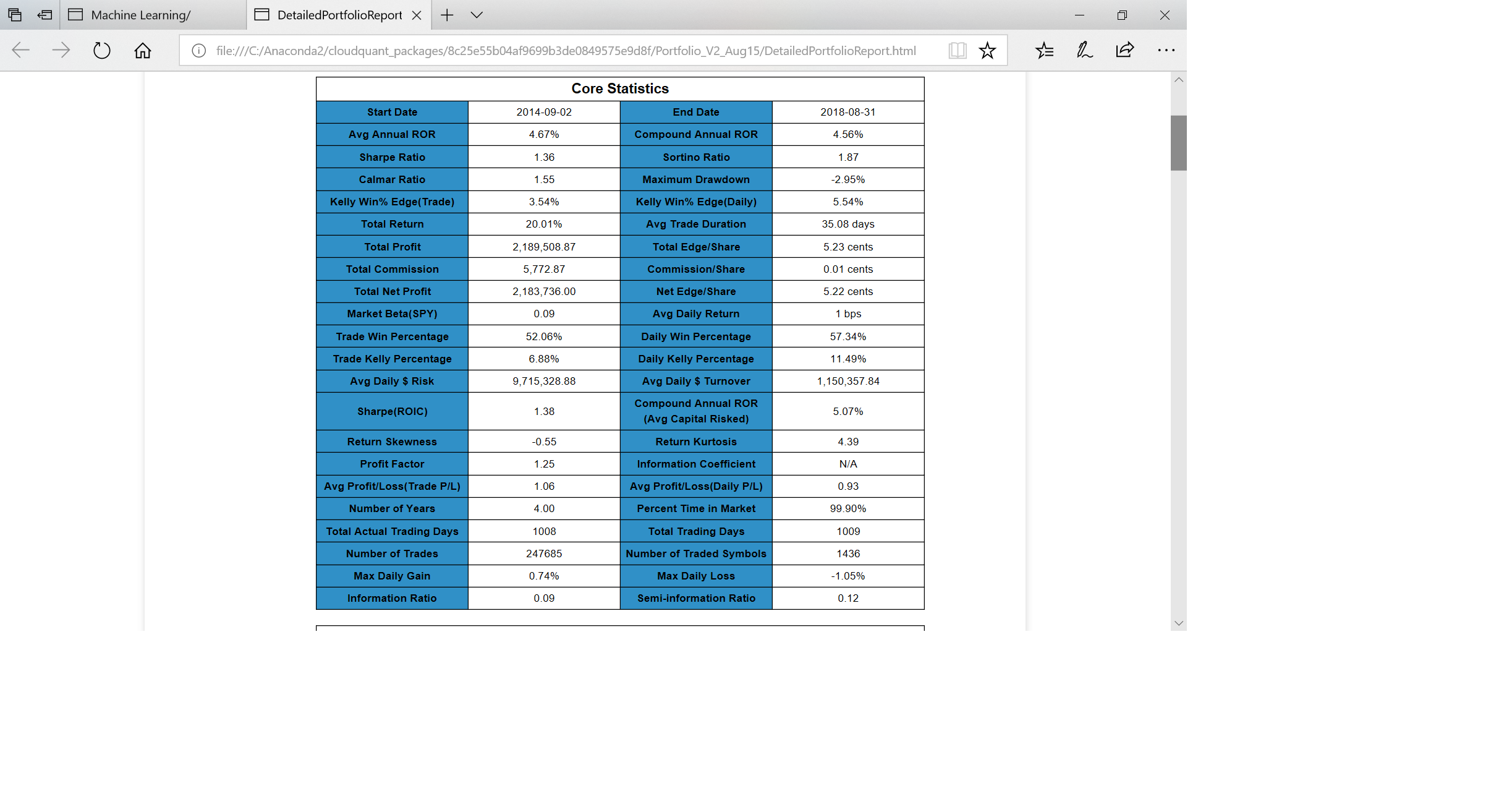
Here are the Core Statistics for the strategy.

My thoughts:

1. Sharpe Ratio of 0.88 on Invested Capital appears realistic for a single factor, especially as I'm using a training / validation split, which reduces overfitting at the expense of less impressive looking backtest statistics.
2. Net Edge/Share of 6.8 cents looks good for a $10 million notional (as in, there's some margin for error in live trading).

aj165602

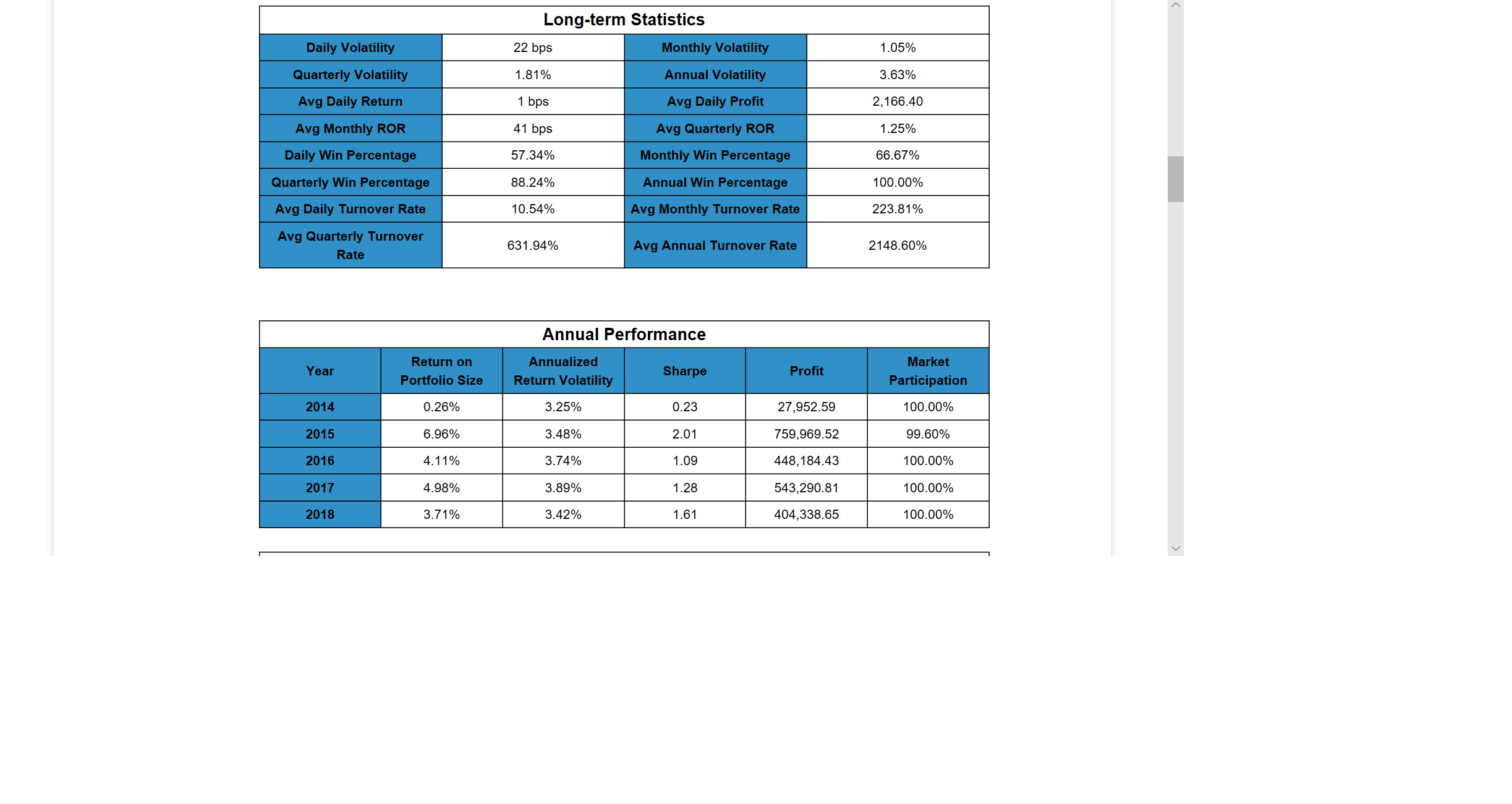
Here are the Long-Term statistics.

My thoughts:

1. Quarterly win percentage of 76% looks solid.
2. Daily turnover of 10% doesn't look excessive,and makes the strategy more likely to carry over to live trading.

aj165602

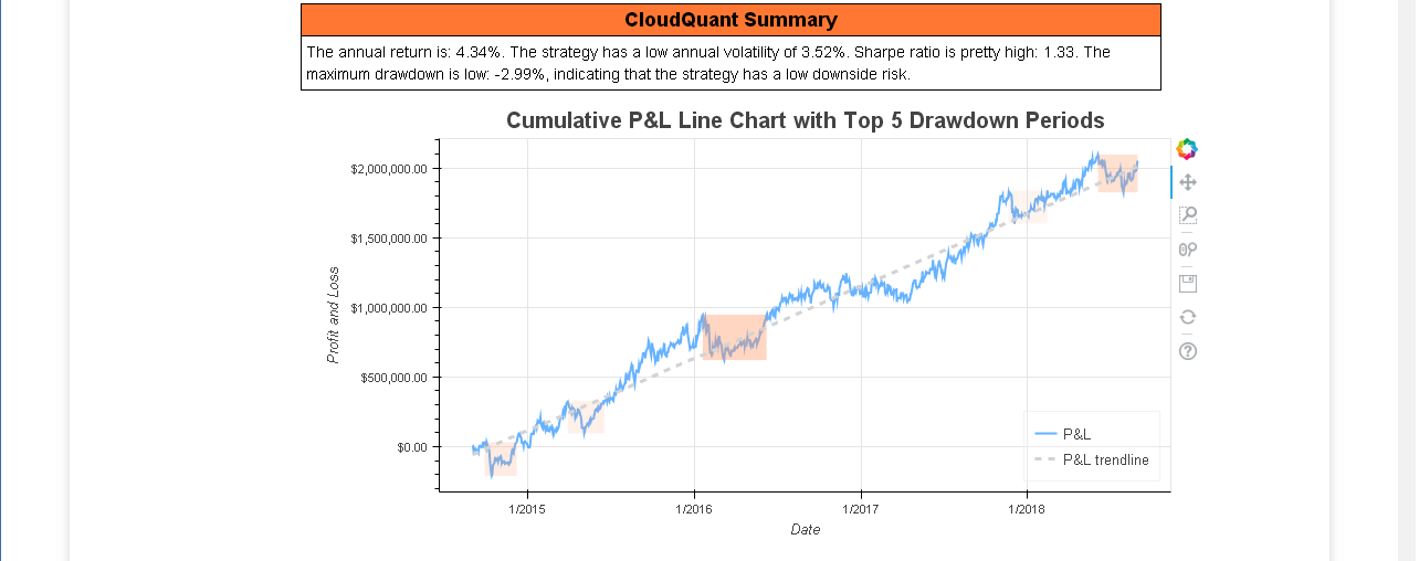
Finally, the CloudQuant summary chart.

My thoughts:

1. Overall trend is good.
2. The large drawdown in 2016 is the main weakness of the strategy. I anticipate that this problem is best overcome through factor diversification.
   

aj165602

The next step is to find another factor that offers something different in terms of underlying economic hypothesis.

This could be another price-based factor that complements the current one, or a completely distinct factor using alternative or fundamental data.

I will examine the complementary factor first, at the same time developing my script to handle two factors.

aj165602

Today's diary is about alpha and beta.

My objective is to create zero-beta strategies, as the value for institutional investors lies in alpha.

It's also important in correctly discarding (and keeping) the appropriate risk factors, as many have a non-negligible positive or negative correlation with the stock market.

Hopefully, I'll be able to demonstrate this in the next Trading Report.

ptunney

AJ, those two periods are the same two periods I ask people to specifically test their models against.

The November 2015 to February 2016 move is the US presidential election cycle.

SPY dropped from 209.97 to 182.86, a 13% drop.

If your drop is less than 13% then console yourself with the fact that you are beating the market.

Pulling symbol data from the same period. Over $1, Over 100k avg vol gives you...

4060 symbols (I did not exclude ETFs)
Average move, down ~30%
2699 symbols down more than 10%
737 symbols down less than 10%
392 symbols up less than 10%
232 symbols up more than 10%

That is the market move you are up against.

This is the quick bit of code I used to get the data. I ran on 2/11/2016 (the day after the down move ended) and just ran it from 09:15 to 09:16 as I just needed to grab historical bars.
By running it in is_symbol_qualified and then returning False it runs nice and fast.

# Gather data for research
# Scope of research : When SPY dropped 13% from Nov 2nd 2015 to Feb 2nd 2016, which stocks went the other way?
# Run on 2/11/2016 09:15 to 09:16 (SPY low after Presidential election was 2/10/2016) 
# Pull 69 bars to go back as far as the recent high point on 11/3/2015
# Get Open for every symbol for 2/10/2016 and 69 days before.

from cloudquant.interfaces import Strategy, Event

class quick_daily_bars(Strategy):

    @classmethod
    def is_symbol_qualified(cls, symbol, md, service, account):  
        myavol = md.stat.avol
        if md.stat.prev_close>1 and myavol>100000:
            mybars=md.bar.daily(start=-69) # grab all the bars.
            mylen=len(mybars.open) # If I asked for len(mybars) I would get 16 because there are 16 lists within the bar data, I ask for the length of just the open prices
            if mylen==69:
                # if I use mybars.open I get all the bars, I want just the bar for 1 day ago, so [-1], and the oldest bar, I used found out the length of the data and used that to find the one I wanted.
                print symbol,service.time_to_string(mybars.timestamp[-(mylen-1)],format="%Y-%m-%d"),mybars.open[-(mylen-1)],service.time_to_string(mybars.timestamp[-1],format="%Y-%m-%d"),mybars.open[-1]
        return False

In the future researchers will use CloudQuant.AI to get this kind of data.

aj165602

Thank you, Paul.

From a researcher's point of view, one of the most compelling reasons to use CQ is the ability to apply modern statistical techniques, as hopefully I'll illustrate in the next few posts.

In the following Trading Report, I have used the same risk factor, but this time I use resampling techniques. I only calculate the resampling estimates on the 3-year period from 2014-17; 2018 is kept as a strictly out-of-sample validation set.

aj165602

Here are the core statistics for the entire 4-year period. The statistical estimates are calculated using the first 3 years' data, and I then run the report on the complete sample.

For me, the main stand-out statistic is the Number of traded Symbols, which is now up to 1534. The Sharpe (ROIC) is also up to 1.02, which is good for a single factor.

SPY Beta is 0.09 and the strategy is dollar-neutral.

aj165602

The Long-term Statistics part of the report shows a healthy Quarterly Win Percentage of 76%.

Annual Performance is consistent, which is to be expected having used robustness techniques, and the out-of-sample appears to show that the strategy generalizes beyond the seen data.

aj165602

Finally, I think the CQ Summary shows an equity curve that is tighter around the trendline --- hence the improved Sharpe ratio.

aj165602

The article by Peter Muller that pt120221 provided earlier this week has resonated strongly with me.

I think the key piece of advice was to squeeze as much value out of an individual idea before moving on to combine with other signals.

In my latest model iteration, I still maintain the discipline of training the model over the three-year 2014-2017 period, reserving the one-year 2017/2018 period as a genuine validation set.

In this iteration, I manage many more risks, which leads to a reduced strategy volatility (3.52% p.a.), but a greatly increased Sharpe ratio (1.33).

aj165602

Looking at the CloudQuant Summary Report, the annual return (4.34%) now exceeds the maximum drawdown (-2.99%). This relationship was also mentioned in the Muller article in the context of autocorrelation of strategy returns.

aj165602

I took a very disciplined approach in developing this more complex model, reconciling the results against another simple model by 'masking' a sequence of variables until I was completely satisfied that both scripts produced the same results under the same conditions.

aj165602

I made a modification to the simulation routine I use, which has had a marginal impact on the performance of the strategy.

Core Stats: Sharpe (ROIC) up to 1.38 , Calmar Ratio up to 1.55.

aj165602

Long-term stats: the Quarterly Win Percentage is now up to 88%.

aj165602

I've now refined the simulation techniques to replace a few heuristics or rules-of-thumb. I'm now happy that I have a methodologically sound portfolio construction step.

There are still a couple of tweaks I can do at the prediction step, but that's more art than science, and I may be able to address the negative skew in returns at the execution step.

But for the time being, I am happy with the state of this single-factor strategy. When I get time, I would like to combine it with another factor, with the goal of dampening down diversifiable risk.

In the meantime, the following 4 charts present the results for the latest methodology.

aj165602

Page 1 of the results (Core Statistics & ROIC Statistics)

aj165602

Page 2 of the results (Long/Short Statistics & Long-term Statistics & Annual Performance):

aj165602

Page 3 of the results (Monthly Performance):

aj165602

Page 4 of the results (Drawdown Analysis & CloudQuant Summary):

kc975943

Interesting work, AJ. Are you using any external data, or is this purely price/volume data-driven? Also, would you mind reposting the article you are referring to?

aj165602

Thank you, kc. It just uses price data.

aj165602

https://forum.cloudquant.com/discussion/298/proprietary-trading-truth-and-fiction-by-p-muller-quantitative-finance-magazine-8-apr-2010#latest

aj165602

In this strategy, I attempt to boost returns using ensemble learning. The CoreStats show an increase in the Sharpe Ratio (ROIC) to 1.40, and the LongTermStats show that the model continues to generalize well out of sample.

aj165602

Here are the LongTermStats. This is the end of this particular line of investigation for the time being.

aj165602

Not much to report, as I have been busily de-bugging an error in my execution script.

A couple of causes for concern were the Portfolio Size in the trading report being markedly different to the Average Risk, and a failure to close positions even when using aggressive orders.

I recommend delving into the csv files that come with the Trading Report, and making liberal use of Print statements in scripts.

aj165602

A good end to the week. To test whether my code is working as expected, I designed an algorithm that combines factors to produce a zero-beta strategy, running for the year ending August 2015.

These are the two main tests satisfied by the report:

1) Should be zero-beta: YES --- 0.00! (This is an item in the Report under the name Market Beta (SPY) )

2) No open positions at the end of the multi-day simulation: YES --- no error message at the top of the report!

aj165602

Update: successfully managed to create a zero-beta (well, -0.01!) strategy across a 4-year simulation.

While taking a break, it suddenly occurred to me what the ‘natural’ counterpart to the original strategy is, so that a new zero-beta strategy with real synergy between the two factors can be created.

I will try to develop that model next.

pp794378

@aj165602 said:
The purpose of this thread is to keep a diary of my attempt at developing an institutional-style long/short equity strategy. My motivation is simple: I want to reach my potential, and I think this will help!

What do you mean by institutional-style strategy? Probably something with high Sharpe, zero beta and high capacity?

aj165602

I had in mind a long/short equity strategy hedged with respect to the risk factors in the Fama-French-Carhart asset-pricing model:

• SPY Beta
• SMB
• HML
• Momentum

Given the focus of Cloudquant data sets, it is probably more relevant to attempt to be hedged with respect to SPY Beta in the first instance.